Homogenous null model
Wiegand, Getzin, Hesselbarth
![]()
First, we need to import the spatstat package for
analyzing spatial point patterns. Also, we import the tidyverse package, a
collection of R packages designed for data science.
  library(spatstat)
  library(tidyverse)
If you don’t have the packages already installed, run the following code in order to install them.
install.packages(c("spatstat", "tidyverse"))Exercise 1
Task: Using the data set DouglasFir_LiveDead_OGN.dat, calculate the O-ring statistic and the L-function. Here, pattern 1 gives the locations of living trees and pattern 2 gives the locations of dead trees. Comparing the univariate measures \(O_{11}(r)\) and \(L_{11}(r)\), how do they differ?
First, we need to import the data using read_delim()
(make sure the data is in your working direction. See
?getwd()/?setwd() for help). The columns are
separated by a semicolon. By using read_delim(), the class
of the data is automatically a tibble (an ‘advanced’
version of a data.frame. For more information see
?tibble).
  douglas_fir <- read_delim(file = "Data/DouglasFir_LiveDead_OGN.txt",
                            delim = ";")

  class(douglas_fir)
## [1] "spec_tbl_df" "tbl_df"      "tbl"         "data.frame"
Print the data. The tibble contains 668 rows (one for
each tree) and 3 columns (x-coordinate, y-coordinate and the marks).
print(douglas_fir, collapse = TRUE)## # A tibble: 668 × 3
## x y mark
## <dbl> <dbl> <dbl>
## 1 69.9 43.9 1
## 2 10.2 60.1 1
## 3 50.4 25.5 1
## 4 40.1 1.03 1
## 5 40.7 15.7 1
## 6 54.2 0.382 1
## 7 41.8 46.3 1
## 8 59.8 28.0 1
## 9 75.7 69.2 1
## 10 48.6 14.1 1
## # ℹ 658 more rowsWe want to edit the column ‘mark’ in a way that 1 == ‘alive’ and 2 ==
‘dead’. We are using two functions of the dplyr package.
mutate() creates a new column (actually we overwrite the
already existing column ‘mark’) and case_when() classifies
the data. Lastly, we convert the column as factors.
  douglas_fir <- mutate(douglas_fir,
                        mark = case_when(mark == 1 ~ "alive",
                                         mark == 2 ~ "dead"),
                        mark = as.factor(mark))
Now, we need to convert the tibble to the
ppp class of the spatstat packages. Firstly,
using ripras(), we need to specify our plot area
(spatstat calls this observation window). The function
calculates a window based on the provided x- and y-coordinates (the
results is returned as a owin object). We can specify the
shape of the window using the shape argument. Secondly, we
convert the tibble to a ppp. The
tibble contains the coordinates and the marks as columns
and we just need additionally to specify the observation window using
the just created owin object.
Plotting the pattern to control it is always a good idea. The plot
function automatically modifies the points according to their mark. Also
the summary() function returns many helpful information
about the point pattern. The functions returns the intensity,
information about the marks (in this case the frequencies, proportions
and intensities of the discrete classes) and information about the plot
area.
  plot_area <- ripras(x = douglas_fir$x, y = douglas_fir$y,
                      shape = "rectangle")

  douglas_fir_ppp <- as.ppp(X = douglas_fir, W = plot_area)

  summary(douglas_fir_ppp)
## Marked planar point pattern:  668 points
## Average intensity 0.07283247 points per square unit
##
## Coordinates are given to 3 decimal places
## i.e. rounded to the nearest multiple of 0.001 units
##
## Multitype:
##       frequency proportion  intensity
## alive       336   0.502994 0.03663430
## dead        332   0.497006 0.03619817
##
## Window: rectangle = [-0.12483, 104.12783] x [-0.1185, 87.8575] units
##                     (104.3 x 87.98 units)
## Window area = 9171.73 square units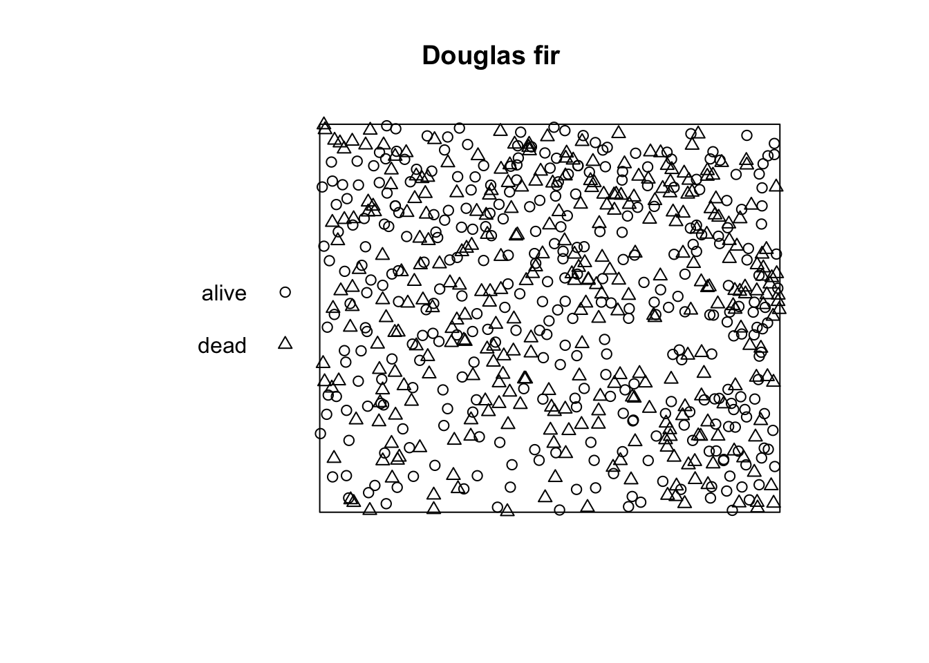
spatstat provides most summary functions for spatial
point pattern analysis (see e.g. ?Kest()). The result is
always a fv object (function value). Almost all summary
functions allow you to specify the edge correction
(correction) and the distances r (r). But
first, we subset the data because we want only to use the ‘alive’ trees
at the moment.
  alive <- subset(douglas_fir_ppp, marks == "alive")

  l_fct_alive <- Lest(X = alive, correction = "Ripley",
                      r = seq(from = 0, to = 45, by = 0.5))
  class(l_fct_alive)
## [1] "fv"         "data.frame"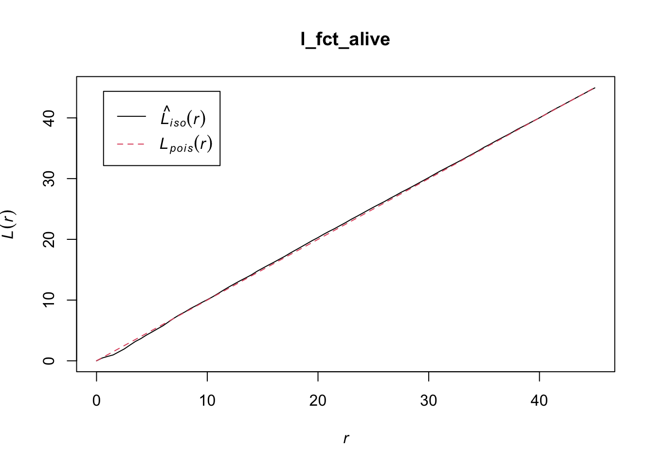
However, as you can see in the plot, Besag’s L-function is not
centered to 0. Also, the O-ring statistic is not available in
spatstat. Therefore, we need to write our own functions.
For that, eval.fv() is quite handy. The function evaluates
expression involving one or more fv objects
(divisor = "d" is just a little trick to improve the bias
of the estimator when r is close to zero).
Lest.cent <- function(input, correction = "Ripley", r = NULL, ...){
l_fct <- Lest(input, correction = correction, r = r, ...)
r <- l_fct$r
eval.fv(l_fct - r)
}
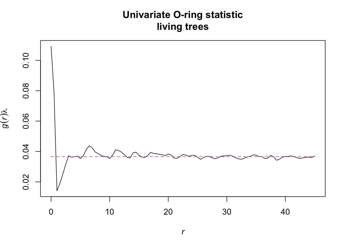
Oest.calc <- function(input, r = NULL, correction = "Ripley", divisor = "d", ...){
p_fct <- pcf.ppp(input, r = r,
correction = correction, divisor = divisor, ...)
lambda <- intensity(unmark(input))
eval.fv(p_fct * lambda)
}Now, we can calculate the summary functions and plot them.
  l_function <- Lest.cent(input = alive,
                          r = seq(from = 0, to = 45, by = 0.5))

  oring_statistic <- Oest.calc(input = alive,
                               r = seq(from = 0, to = 45, by = 0.5))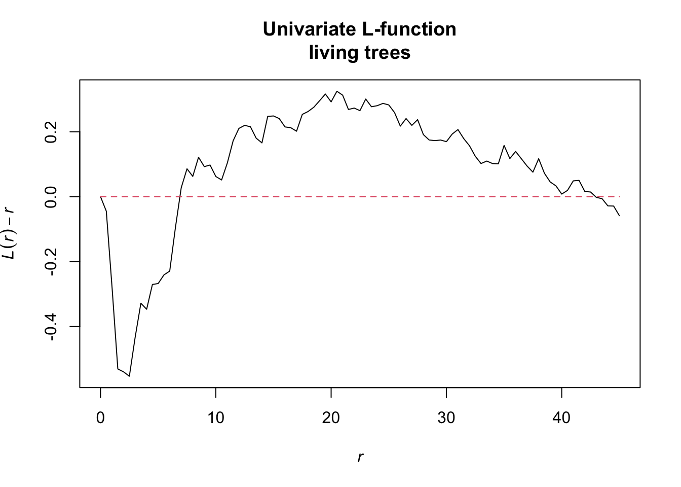
Alternatively, these functions are already implemented in the onpoint
package (Hesselbarth 2025), a small collection of utility functions
based on spatstat.
  # install.packages("onpoint")
  library(onpoint)

  l_function <- center_Lest(x = alive, r = seq(from = 0, to = 45, by = 0.5))

  oring_statistic <- Oest(x = alive, r = seq(from = 0, to = 45, by = 0.5))
Exercise 3
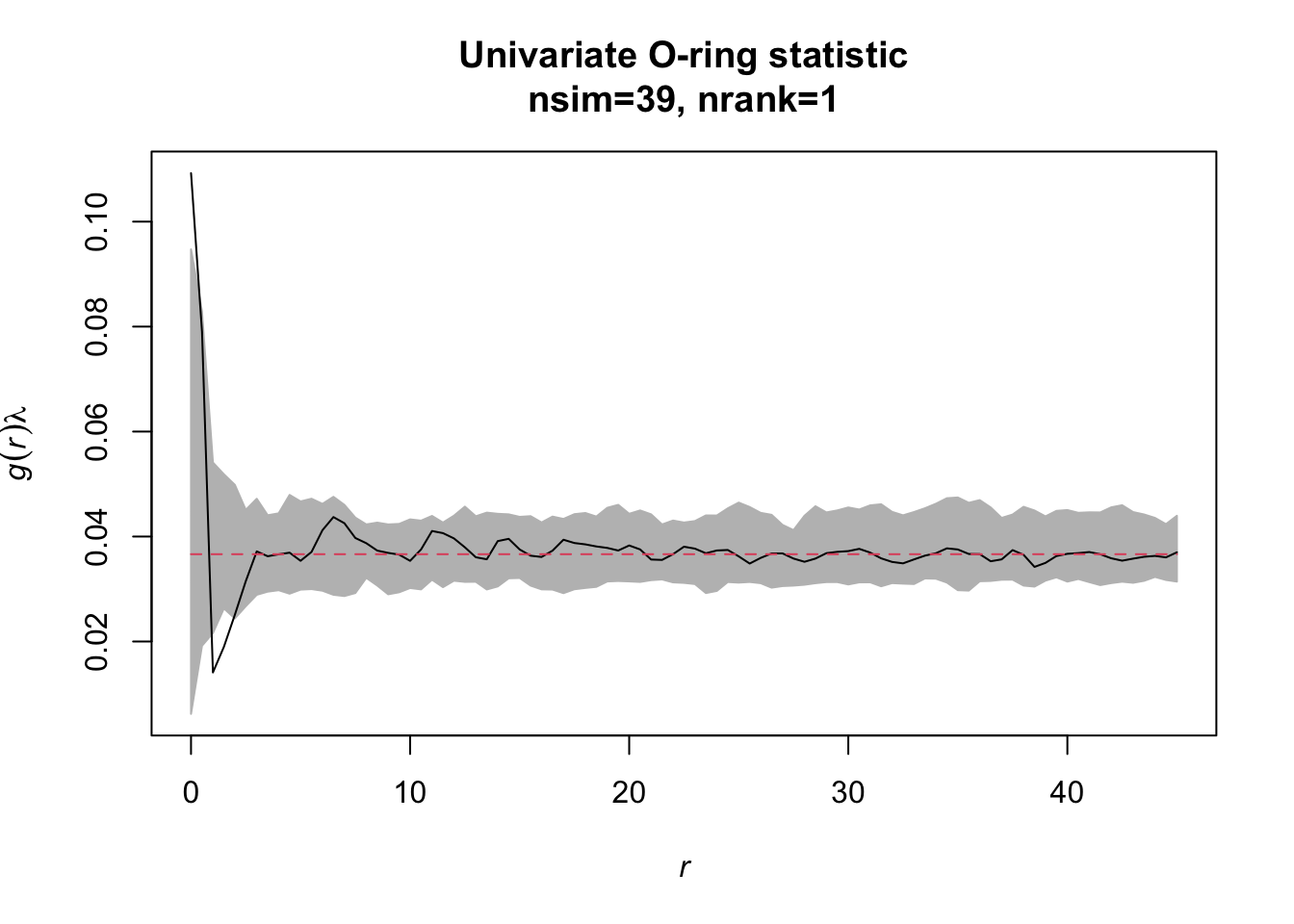
Task: Redo the analysis but now with simulation envelopes. How does the simulation envelope change if you change the settings for the envelope from # simulations=39/‘lowest/highest’=1 to simulations=199/‘lowest/highest’=5.
The function envelope of the spatstat
package calculates simulation envelopes. The number of simulations can
be specified with the argument nsim, the lowest/highest
values with the argument rank. When not specified
otherwise, the functions uses ‘CSR’ as null model. The fun
argument can handle any summary function that spatstat
provides (or the ones we implemented as long as they return a
fv object).
simulation_envelope_39 <- envelope(Y = alive, fun = Oest.calc,
r = seq(from = 0, to = 45,
by = 0.5),
nsim = 39, nrank = 1)
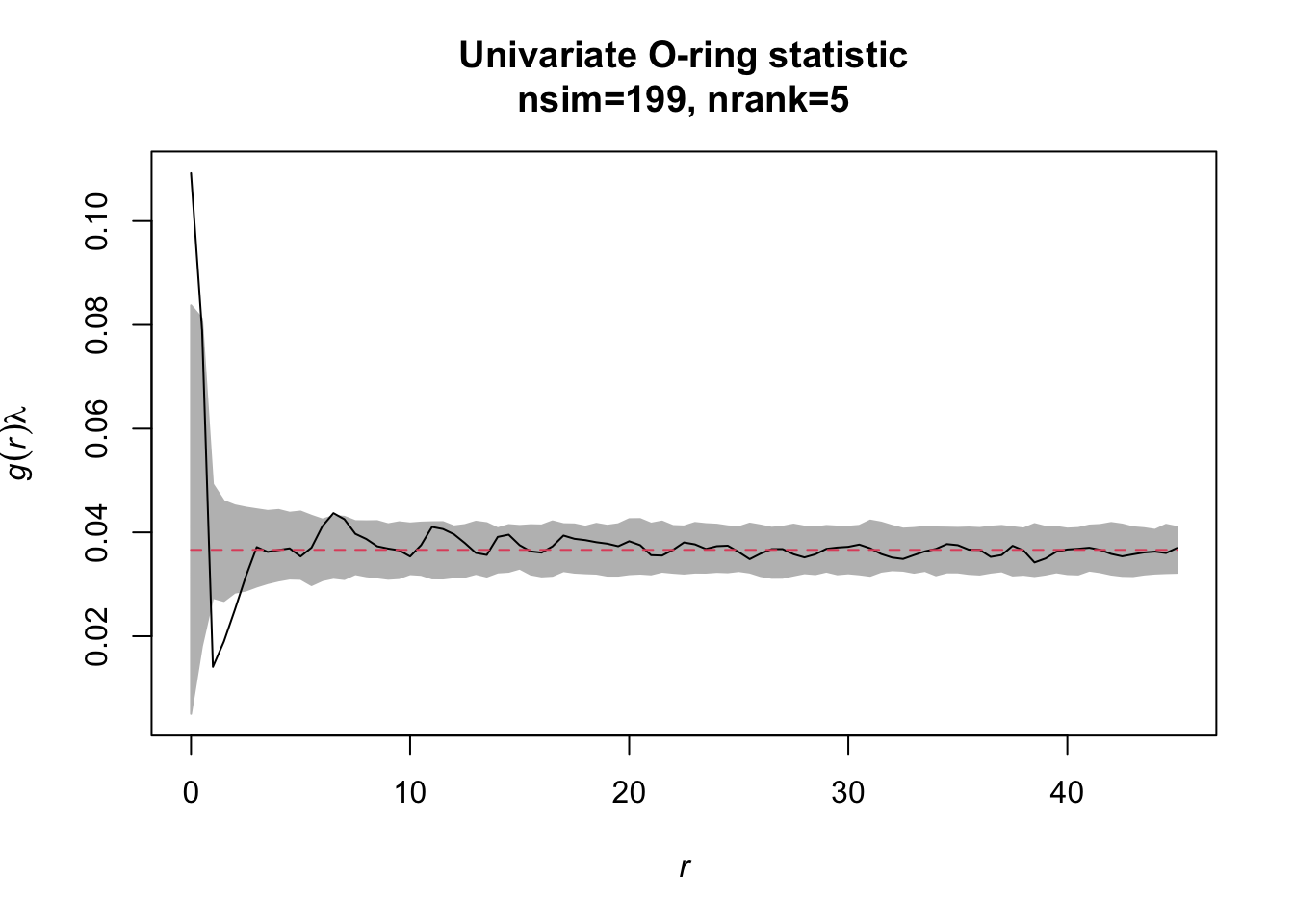
simulation_envelope_199 <- envelope(Y = alive, fun = Oest.calc,
r = seq(from = 0, to = 45,
by = 0.5),
nsim = 199, nrank = 5)The null model ‘CSR’ basically just simulates pattern with the same number of events using a Poisson process, i.e. using random coordinates within the study plot with a homogenous intensity and no interaction between events.
Just use the plot() function to display the results.
Exercise 4
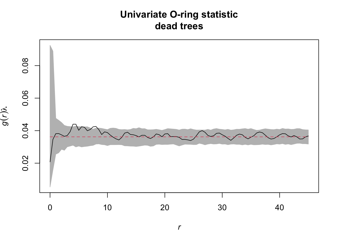
Task: Also look at the functions O22(r) and L22(r). Is there a striking difference between dead and alive Douglas fir trees?
So this time, we want to subset all ‘dead’ trees.
  dead <- subset(douglas_fir_ppp, marks == "dead")

  simulation_envelope_dead <- envelope(Y = dead, fun = Oest.calc,
                                       r = seq(from = 0, to = 45,
                                               by = 0.5),
                                       nsim = 199, nrank = 5)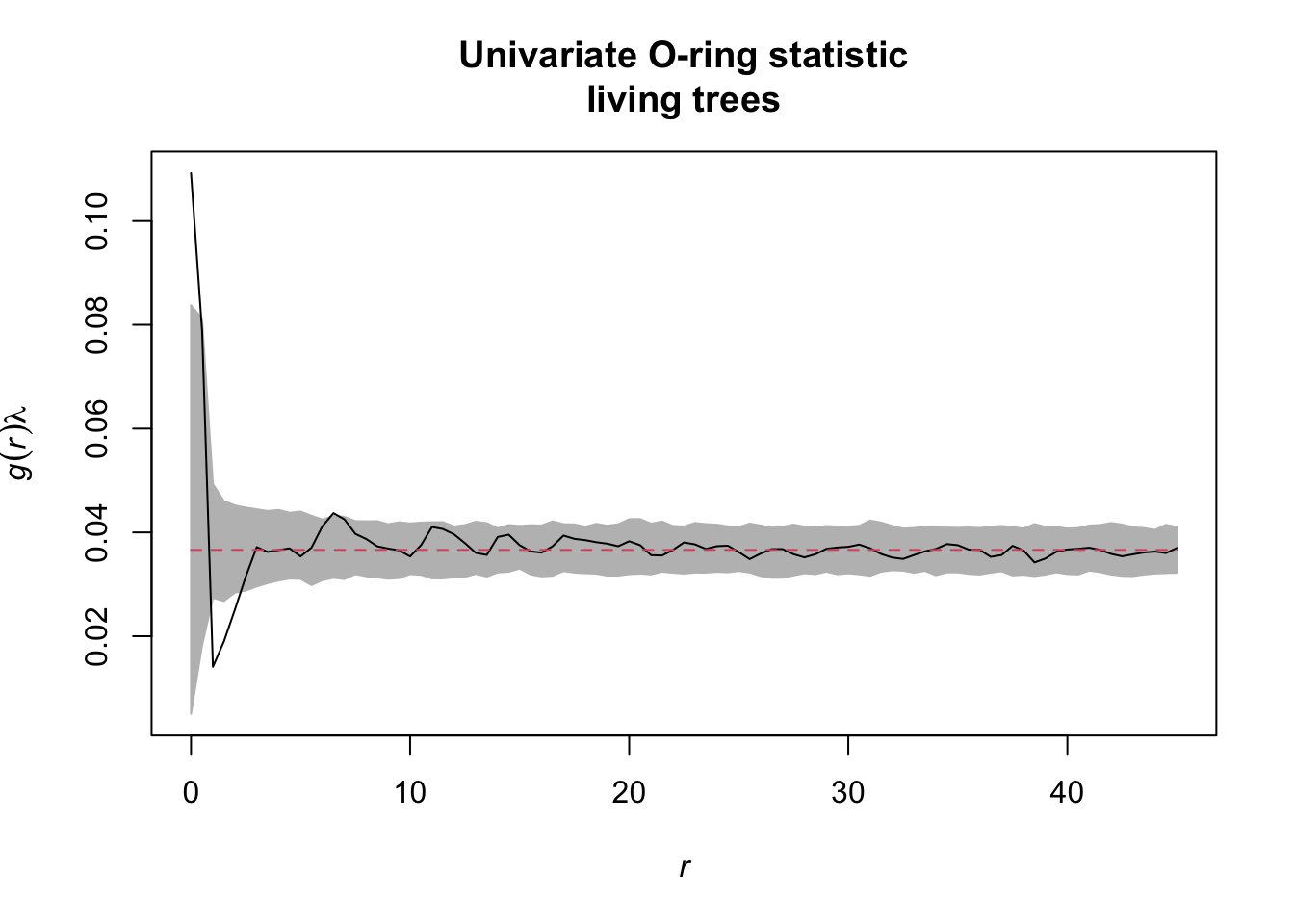
…some more
onpoint also provides a plotting function for
envelope objects. Similar to spatstat, the
simulation envelopes as well as the observed value are included,
however, so-called ‘quantum bars’ indicate the location of the observed
value in relation to the envelopes.
  plot_quantums(simulation_envelope_199,
                xlab = "r [m]", ylab = "O(r)",
                title = "Univariate O-ring statistic\nliving trees",
                base_size = 7.5)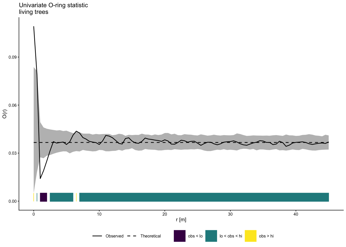
References:
Baddeley, A., Rubak, E., Turner, R., 2015. Spatial point patterns: Methodology and applications with R. Chapman and Hall/CRC Press, London.
Getzin, S., Dean, C., He, F., Trofymow, J.A., Wiegand, K., Wiegand, T., 2006. Spatial patterns and competition of tree species in a Douglas fir chronosequence on Vancouver Island. Ecography, 29, 671-682.
Getzin, S., Wiegand, T., Wiegand, K., He, F., 2008. Heterogeneity influences spatial patterns and demographics in forest stands. J. Ecol. 96, 807-820.
Hesselbarth, M.H.K. (2025). onpoint: Helper Functions for Point Pattern Analysis. R package version 1.1, https://CRAN.R-project.org/package=onpoint.