Cluster processes / Mark correlation function / Heterogenous conditions
Wiegand, Getzin, Hesselbarth
You can find a link to download the data here. The .zip-folder
includes two sub-folders, in which you can find the same datasets
formatted for both Programita (filename extension
.dat/.mcf) and R (filename extension
.txt).
Especially when using Programita, but also using R, make screenshots of your results (or save the results to your disk in any other way) for the plenum discussion later.
For more information/background, please see Homo_NullModels.pptx.
Cluster process
For more information, please see Slides 155 ff.
Exercise 1)
Perform a point-pattern analysis on the Hemlock_Adults_vs_SmallSaps data set using CSR as null model. We are now especially interested in pattern 2, the small saplings. Using a cell size of 1 meter, calculate the \(O_{22}(r)\). Up to which scale do we find significant clustering of the saplings?
Exercise 2)
Use the pair-correlation function to fit a cluster process to the saplings data and use the fitted model to simulate null model data. Is the null model suitable for the field data?
Exercise 3)
If the \(O_{11}(r)\) function falls into the new envelope, you fitted good parameters for the cluster process. Have a look at the fitted parameters. Here, the typical cluster size and number of parents are of interest.
Exercise 4.)
Looking at the pattern of adult trees and saplings, is the fitted value for the number of parents realistic? If not so, what could be the reason?
Mark correlation function (Stoyan’s \(k_{mm}\))
Exercise 1)
The data set Alive_DouglasFir_OGN contains the location and stem diameters (diameter at breast height, DBH) for all live Douglas fir trees in the Old-growth North plot. Calculate the mark-correlation function for the DBH. What do these results suggest?
Exercise 2)
Calculate simulation envelopes to test for significance. As a null model use random labelleing. What could be a possible ecological explanation of your results?
Inhomogeneous point patterns
Exercise 1)
In the data set Hemlock_Adults_vs_SmallSaps, you can observe a clear gradient in the density of adult trees. Calculate \(O_{11}(r)\) and \(L_{11}(r)\) for pattern 1 (adult trees) to see up to which scale clustering of the trees can be observed using CSR as null model.
Exercise 2)
Getzin et al. (2008) show that the study area is heterogenous. We are going to account for this heterogeneity by fitting a heterogeneous Poisson processes. Estimate \(\lambda(x,y)\) and plot a map of the results. The gradient should be well visible.
Exercise 3)
Use the previously estimated intensity \(\lambda(x,y)\) to simulate a heterogenous Poisson process. Does \(O_{11}(r)\) now fit into the simulation envelope? How do you interpret the result?
## Warning: The `<scale>` argument of `guides()` cannot be `FALSE`. Use "none" instead
## as of ggplot2 3.3.4.
## This warning is displayed once every 8 hours.
## Call `lifecycle::last_lifecycle_warnings()` to see where this warning was
## generated.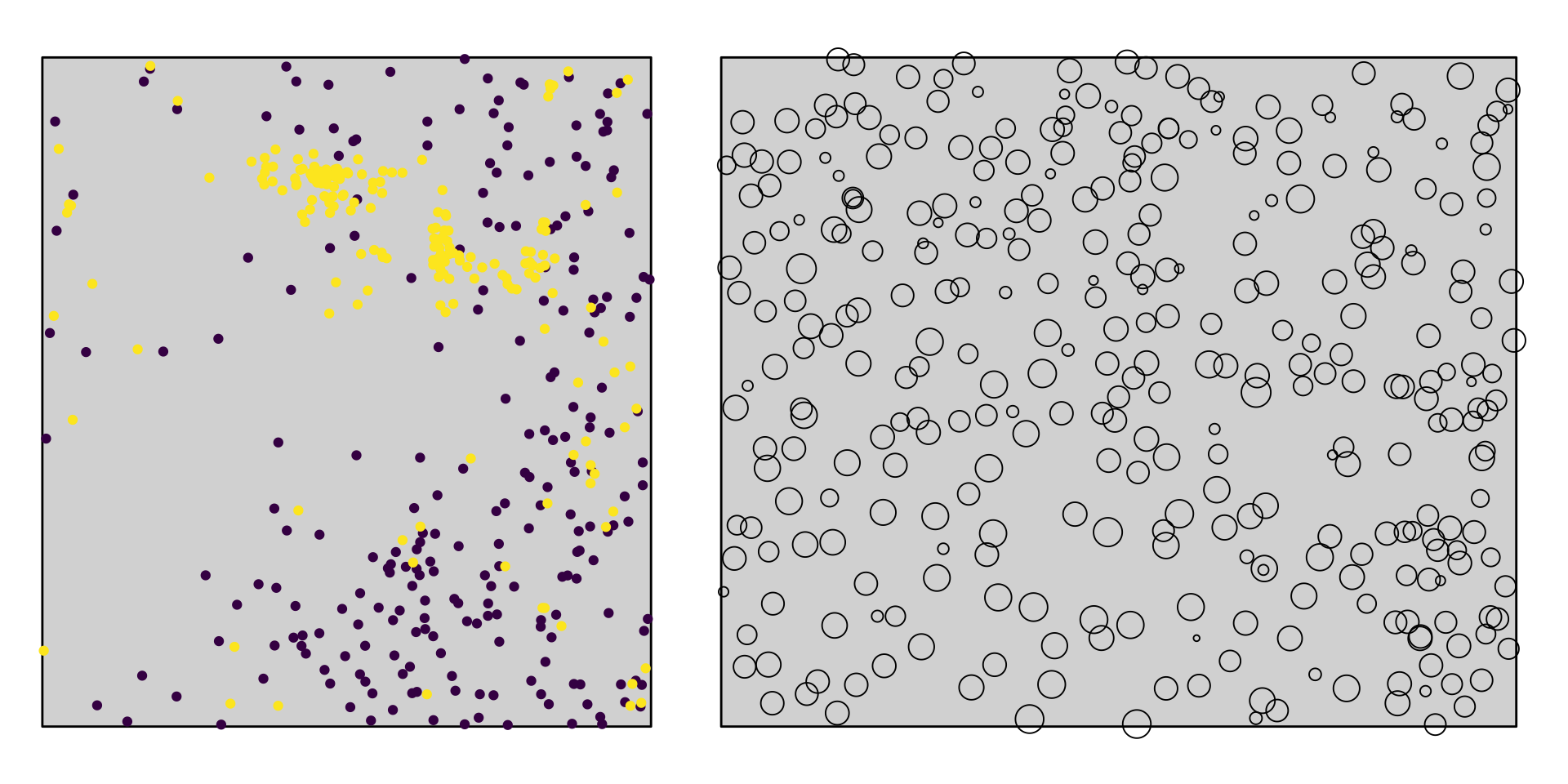
Softcore- and Hardcore Process
Exercise 1)
For this, use the data set DouglasFir_LiveDead_OGN.dat again.
Can the small-scale regularity in the living Douglas fir trees be modeled by a hard-core process? What about a soft-core process?
Literature:
Getzin, S., Wiegand, T., Wiegand, K., He, F., 2008. Heterogeneity influences spatial patterns and demographics in forest stands. J. Ecol. 96, 807–820