Homogenous null model

You can find a link to download the data here. The .zip-folder includes two sub-folders, in which you can find the same datasets formatted for both Programita (filename extension .dat/.mcf) and R (filename extension .txt).

Especially when using Programita, but also using R, make screenshots of your results (or save the results to your disk in any other way) for the plenum discussion later.

For more information/background, please see Homo_NullModels.pptx.

Exercise 1)

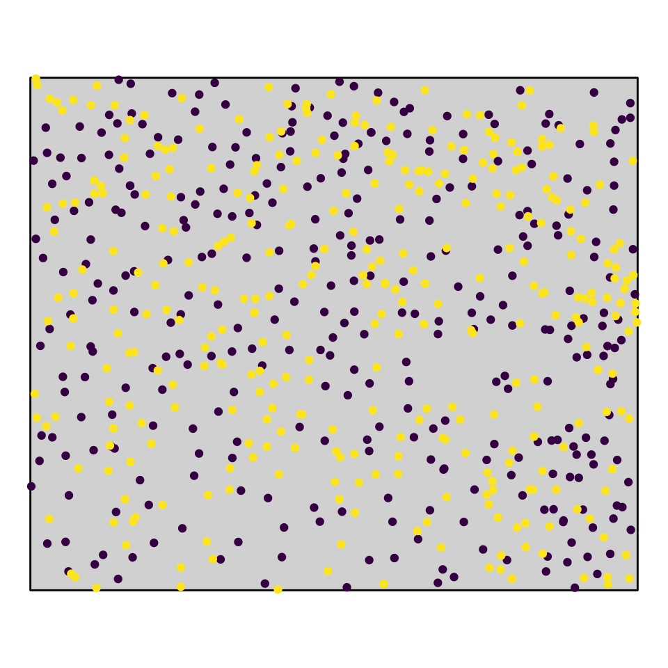
Using the data set DouglasFir_LiveDead_OGN, calculate the O-ring statistic and the L-function. Here, pattern 1 gives the locations of living trees and pattern 2 gives the locations of dead trees. Comparing the univariate measures \(O_{11}(r)\) and \(L_{11}(r)\), how do they differ?

For more information, see Slides 6 ff., Slides 26 & Slides 51 ff.

Exercise 2)

The L-function is said to have a memory effect because of its cumulative nature (counting points within discs instead of circles compared to the O-statistic). Can you see it in your results?

For more information, see Slides 26 & Slides 51 ff.

Exercise 3 )

Redo the analysis but now with simulation envelopes and the null model CSR. How does the simulation envelope change, if you change the number of simulations from n = 39 to n = 199 (using the \(5^{th}\) lowest/highest values).

For more information, see Slides 10 ff. & Slides 51 ff.

Exercise 4 )

Also look at the O-ring statistic \(O_{22}(r)\) and the L-function \(L_{22}(r)\) for all dead trees. Is there a striking difference between dead and living Douglas fir trees? Again, use simulation envelopes and the null model CSR.