Homogenous null model
Wiegand, Getzin, Hesselbarth
You can find a link to download the data here. The .zip-folder
includes two sub-folders, in which you can find the same datasets
formatted for both Programita (filename extension
.dat/.mcf) and R (filename extension
.txt).
Especially when using Programita, but also using R, make screenshots of your results (or save the results to your disk in any other way) for the plenum discussion later.
For more information/background, please see Homo_NullModels.pptx.
Exercise 5)
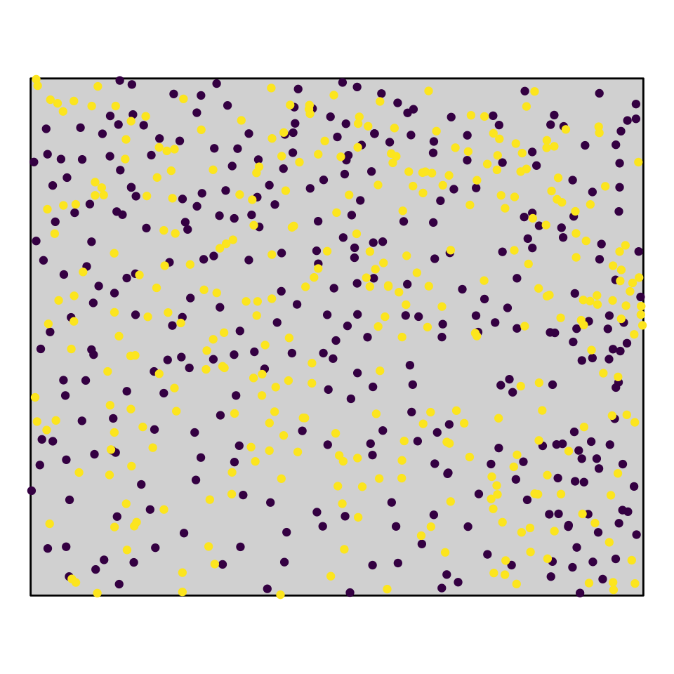
Using the data set DouglasFir_LiveDead_OGN, calculate the bivariate \(g_{12}(r)\) function using the null model random labeling. Was the process that labeled trees as dead or alive a random process?
For more information, see Slide 81 ff.
Exercise 6)
Redo the analysis from 5) and try out different settings for the number of simulations and the used lowest/highest values (e.g. n = 39, 199, 499 and lowest/highest = 1, 5, 10). Do the results change?
For more information, see Slide 81 ff.
Exercise 7)
Now use the data set DouglasFir_Adult_vs_Seedling_OGN. Here, pattern 1 gives the locations of adult trees and pattern 2 gives the locations of seedlings. Calculate \(O_{12}(r)\) and generate 95% confidence envelopes for the null model antecedent conditions (Pattern 1: fixed, pattern 2: random). What would be a meaningful interpretation of the results?
Exercise 8)
How does the interpretation of the ‘Toroidal shift’ null model differ from the null models in 7)? What is the advantage? Is it always an advantage?
For more information, see Slides 94 ff.
