Solution Spatial data
Maximilian H.K. Hesselbarth
2022/10/24
Make sure you can install and load all packages. This includes
terra and sf, but also the
tidyverse.
library(tidyverse)

library(sf)
library(terra)
Next, go to https://www.naturalearthdata.com and download the “Small scale data, 1:110m” > “Cultural” > “Admin 1 – States, Provinces” data set. Additionally, download the “NLCD 2019 Land Cover (CONUS)” data set from https://www.mrlc.gov.
Once you downloaded all the data, read it into your R Session using the corresponding packages.
states <- sf::read_sf("slides/spatial/data/provinces.shp")

nlcd <- terra::rast("slides/spatial/data/nlcd_2019.img")
Make sure both the vector and the raster data have the same CRS (Hint: It’s often faster to project vectors instead of raster. If projecting the raster, have a look at the ‘method’ argument).
states <- sf::st_transform(x = states, crs = terra::crs(nlcd))Next, remove Alaska and Hawaii from the states vector because there is no NLCD data for these states. Next select only the 5 largest states in area
states_large <- dplyr::filter(states, !name %in% c("Alaska", "Hawaii")) |>
  dplyr::mutate(area_m = as.numeric(sf::st_area(geometry))) |>
  dplyr::arrange(-area_m) |>
  head(n = 5)
First plot the NLCD data and add the largest states to the map. Try to use the region as shape fill.
plot(nlcd)

plot(states_large["region"], add = TRUE)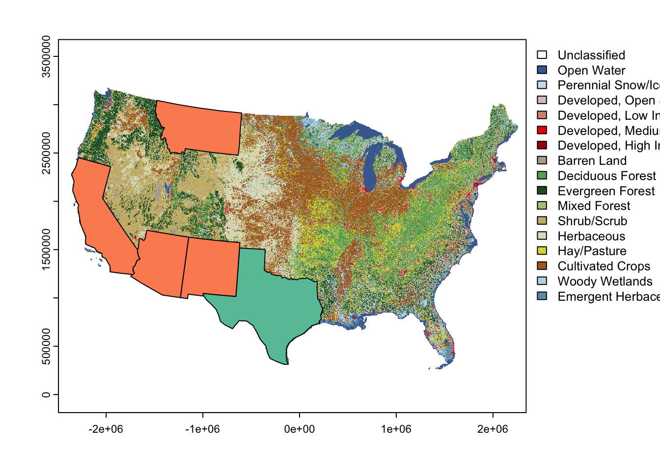
Now, pick one state (your home state, a state you recently visited, a state you want to visit, …) and get the NLCD data for that state only.
kansas <- dplyr::filter(states, name == "Kansas")

nlcd_kansas <- terra::crop(x = nlcd, y = kansas) |>
  terra::mask(mask = kansas)
Next, get all values of the cropped NLCD data and remove all
NA and NaN values. Calculate the relative
amount of all remaining values. Which one is the most dominant
land-cover class in your state?
values_kansas <- terra::values(nlcd_kansas)

values_kansas <- values_kansas[is.finite(values_kansas)]

rel_classes <- sort((table(values_kansas) / length(values_kansas)) * 100,
                    decreasing = TRUE)
Last, try to reclassify the raster into less classes (e.g., use the bigger classification found atNLCD classes)
classes_present <- names(rel_classes)

class_mat <- cbind(as.numeric(classes_present),
                   as.numeric(stringr::str_sub(classes_present, start = 1, end = 1)))

kansas_reclass <- terra::classify(x = nlcd_kansas, rcl = class_mat)